Predictability

Only the primary layer is stimulated by a spatio-temporal input signal. The input signal is supposed sparse, and parameter $m_I^{(1)}$ denotes the input sparsity (the average proportion of neurons which are stimulated at each time). As the number of primary neurons is equal to the number of input channels, the activation signals of primary neurons are strongly correlated with their input signals. If we suppose moreover that the input signal is binary, i.e. $\forall i, \forall t, I_i^{(1)}(t) \in \{0,1\}$, the primary pattern of activation $\mathbf{x}^{(1)}$ and the input signal $\mathbf{I}^{(1)}$ have almost the same values. On the contrary, there is no spatial matching between the primary pattern of activation $\mathbf{x}^{(1)}$ (and/or the input signal $\mathbf{I}^{(1)}$) and the secondary pattern of activation $\mathbf{x}^{(2)}$.

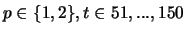Figure 2: Measures of correlations between spatial patterns of activation, in primary and secondary layers, for (random) non-periodic and periodic input signals. The activity of the system is observed between $t=51$ and $t=150$. For $p \in \{1,2\}, t \in 51,...,150$, we measure the correlation between $\mathbf{x}^{(p)}(100)$ and $\mathbf{x}^{(p)}(t)$. $N^{(1)}=200$, $N^{(2)}=200$, other parameters are in Tab.1. - a - Non-periodic input signal, Primary layer, - b - Non-periodic input signal, Secondary layer, - c - Period-5 input signal, Primary layer, - d - Period-5 input signal, Secondary layer.

One can however remark that primary and secondary patterns of activation are not independent (due to the weights couplings between the two layers). In other words, the dynamics that takes place in secondary layer is partly predictable, knowing primary layer activity. This statistical dependency can be observed if our system is submitted to a periodic input signal $\mathbf{I}^{(1)}$ of period $\tau$ so that $\forall t, \mathbf{I}^{(1)}(t+\tau)=\mathbf{I}^{(1)}(t)$ (see Fig.2). In that case, the chaotic dynamics in the secondary layer has a residual periodicity, i.e. $\forall t, \mbox{cor}(\mathbf{x}^{(2)}(t),\mathbf{x}^{(2)}(t+\tau))\simeq 0.6$. This mutual periodicity makes it possible to associate the periodic primary pattern of activation $\mathbf{x}^{(1)}$ to the periodically distributed secondary pattern of activation $\mathbf{x}^{(2)}$ (comparable to a cyclo-stationary random process). So, in case of periodic input signals, primary and secondary layers display a weak dynamical coupling, i.e. one can predict the distribution of secondary layer activations, knowing the primary pattern of activation. This statistical predictability allows to learn spatio-temporal associations between the two layers, and will be used in next section. Note however that secondary layer chaotic dynamics is not equivalent to (and richer than) a random process. Indeed, we have remarked that the distribution of activations in the secondary layer is highly sensitive to small changes on the spatial and temporal characteristics of the input signal. One can observe a strong remapping in the secondary pattern of activation after a little change on the input signal. This denotes a structural instability of the dynamics (a spontaneous tendency to modify its inner dynamical organization). Our system is thus highly sensitive to noise or stimulus variations. It thus behaves in a very different manner than a system composed of stochastic units. We have also remarked that signals with long periods (i.e. $\tau > 10-15$) lead to a secondary pattern of activation whose residual period is an harmonic of the input period. In that case, one can not have bijective associations between primary spatial patterns of activation and secondary spatial distributions of activation. In next sections, we assume that input sequences have rather short periods, of the order of 3-10.