Activation dynamics

Our dynamical system (1) is defined as a pool of $P$ interacting populations of neurons, of respective sizes $N^{(1)}$, ..., $N^{(P)}$. The global number of neurons is $N=\sum_{p=1}^P N^{(p)}$. The synaptic weights from population $q$ towards population $p$ are stored in a matrix $\mathbf{J}^{(pq)}$ of size $N^{(p)}\times N^{(q)}$. The state vector of population $p$ at time $t$ is $\mathbf{x}^{(p)}(t)$, of size $N^{(p)}$. The initial conditions $x_i^{(p)}(0)$ are set according to a random draw uniform in $]0,1[$. At each time step $t\geq1$, $\forall (p,q) \in \{1,..,P\}^2$, $\forall i \in 1,...,N^{(p)}$,

$$h_i^{(pq)}(t)=\sum_{j=1}^{N^{(q)}}J_{ij}^{(pq)} x_j^{(q)}(t-1)$$

is the local field of population $q$ towards neuron $i$ of population $p$. This variable measures the influence of a particular population on the activity of a given neuron. We also consider spatio-temporal input signals $\mathbf{I}^{(p)}=\{\mathbf{I}^{(p)}(t)\}_{t=1..+\infty}$, where $\mathbf{I}^{(p)}(t)$ is a $N^{(p)}$ dimensional input vector at time $t$ on population $p$. The input $\mathbf{I}^{(p)}(t)$ acts like a bias on each neuron (on the contrary to Hopfield system, the input doesn't correspond to the initial state $x_i^{(p)}(0)$ of the network). Then, the global equation of the dynamics is :

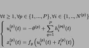$$\begin{array}{l} \forall t\geq 1, \forall p \in \{1,...,P... ...)}(t)+I_i^{(p)}(t)\right)} \end{array} \right. \end{array}$$ (1)

The activation potentials $u_i^{(p)}$ have real continuous values, and correspond to a linear combination of afferent local fields minus activation threshold $\theta^{(p)}$. The activation states $x_i^{(p)}(t)$ are continuous and take their values in $]0,1[$, with a nonlinear transfer function $f_g(u)=({1+\tanh(gu)})/{2}$, whose gain is $g/2$. We call ``pattern of activation'' the spatio-temporal signal $\mathbf{x}^{(p)}$ corresponding to the exhaustive description of a trajectory of the system's dynamics in layer $p$. An important characteristics of our system is the random nature of the connectivity pattern. We suppose that the distribution of the connection weights follow the Gaussian law $\mathcal{N}(0,{(\sigma_J^{(pq)})^2}/N^{(q)})$, so that $E\left(\mbox{var}\left(\sum_{j=1}^{N^{(q)}}J_{ij}^{(pq)}\right) \right)=(\sigma_J^{(pq)})^2$. This random draw implies that our synaptic weights are almost surely non-symmetric. This non-symmetry is a necessary requirement for having complex dynamics. As the local fields $h_i^{(pq)}$ are updated synchronously, the global dynamics (1) also obeys to a synchronous update. Then, the state of the system at time $t$ both depends on the state of the system at time $t-1$ and the input $\mathbf{I}(t)$ (at time $t$). One can thus notice that (i) the transmission delay is uniformly equal to 1, (ii) our system is deterministic as soon as the input signal is set according to a deterministic process.