Capacity

The number of different spatial input patterns that can be memorized in recurrent attractor systems, like Hopfield systems, is generally found to be linearly dependent in $N$. One thus defines a capacity criterion $\alpha_c={n_c}/{N}$ where $n_c$ is the maximal ``critical'' number of spatial patterns that can be learned. For a given value of $N$, when one tries to learn more than $\alpha_c N$ spatial patterns, the retrieval ability suddenly decreases (``catastrophic'' forgetting). Starting from a tabula rasa, one can also store spatio-temporal periodic patterns instead of spatial patterns in recurrent systems [19]. Basically, individual neurons work as coincidence detectors, and tend to react specifically to the co-activation of a given set of pre-synaptic neurons. Globally, one can observe chains of firing, leading to a stable spatio-temporal activation pattern [17]. In case such chains are closed, every different loop corresponds to a different periodic (cyclic) attractor. The capacity of such systems obey to the same constraints as Hopfield systems, and is also defined as the number of spatial patterns that can be stored, independently of their temporal succession. Theoretical estimates of the capacity of such systems can be found in [24,17]. In our systems, there is no explicit storage of spatio-temporal sequences. The retrieval relies on two mechanisms: (i) the decrease of chaos (i.e. increase of predictability) between primary and secondary layers activities (which is necessary for the robustness of the response) and (ii) a coincidence detection mechanism from secondary layer towards primary layer (which activates or disables feedback signal). In order to allow comparison with existing models, we define a measure of capacity that relies on this retrieval mechanism. The ``knowledge'' of a given sequence of inputs thus manifests in the network ability to activate a feedback signal which is coherent with the input signal. For an estimation of the capacity, we only refer to the size of the secondary layer $N^{(2)}$, as the size of primary layer has no influence on the retrieval properties of the system. During the training process, a spatio-temporal sequence $\mathbf{s}_1$ is repeatedly presented until our learning mechanism (2) produces an active feedback signal. Then, we test the correlation between input and feedback signals for that particular sequence (with dynamics (1)), i.e. $\forall t>0, r_{1,1}(t)=\mbox{cor}(\mathbf{I}^{(1)}(t),\mathbf{F}^{(12)}(t))$ and $\hat{r}_{1,1}=(1/T) \sum_{t=1}^T r_{1,1}(t)$, with $T»1$. If $\hat{r}_{1,1}$ is close to 1, input and feedback signals are found to overlap. Then a second sequence is learned, then a third one, ..., then a $k^{th}$ one... The period of the $k^{th}$ sequence is chosen between 3 and 7, i.e $\tau_k \in \{3,4,5,7\}$, with equal probability. At step $k$, we measure the retrieval for every previously learned sequence, i.e for $m=1..k$, we calculate $\hat{r}_{m,k}$. For every value of $k>0$, the total number of spatial patterns that compose the learned sequences is equal to $n_k=\sum_{m=1}^k \tau_m$. The mean retrieval among all learned sequences is equal to $\hat{r}_k=(1/k)\sum_{m=1}^k \hat{r}_{m,k}$. When $\hat{r}_k$ is close to one, the retrieval is good for almost every sequence. When $\hat{r}_k$ is close to zero, the ability to retrieve any of the learned sequences is null, which corresponds to a ``catastrophic forgetting''.

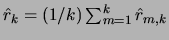
Figure: Different measures of the capacity of the model. $\hat{r}_k$ is plotted in function of $n_k$ (see text). Non-specified parameters are in Tab. 1. - a - Inter-individual variability, in case of elementary sequences learning, with $\varepsilon ^{(12)}=0.1$, $\varepsilon ^{(22)}=0$ and $N^{(2)}=200$. Dotted lines correspond to individual networks, plain line corresponds to the mean over the 10 networks. - b - Measures of capacity for different values of $\varepsilon ^{(22)}$, in case of elementary sequences learning, with $\varepsilon ^{(12)}=0.1$, and $N^{(2)}=200$. - c - Measures of capacity for different values of $N^{(2)}$, in case of elementary sequences learning, with $\varepsilon ^{(12)}=0.1$ and $\varepsilon ^{(22)}=0.02$. - d - Measures of capacity for different values of input sparsity $m_I^{(1)}$, with $\varepsilon ^{(12)}=0.1$, $\varepsilon ^{(22)}=0.02$ and $N^{(2)}=200$.

This experiment has been carried out on 10 networks (Fig.7-a-) with elementary sequences (and without overlap between the spatial patterns composing the sequences). The size of secondary layer is $N^{(2)}=200$ and learning only takes place on feedback links (i.e. $\varepsilon ^{(22)}=0$). For every network, $\hat{r}_k$ is plotted in function of $n_k$. Globally, the shape of the curves is similar for every network, with good retrieval for low values of $n_k$, and a sudden decrease towards zero. So, one can estimate, for a given network, a critical value $n_c$ (corresponding to the sudden decrease) so that $\alpha_c=n_c/N^{(2)}$. There are sensitive differences between individual networks (i.e. $n_c$ is between 120 and 180), and the mean capacity $\alpha_c$ is found to be of the order of 0.7. The shape of the curves and the value of $\alpha_c$ strongly vary depending on the parameters settings. We have tried on the following experiments to estimate the role of $\varepsilon ^{(22)}$ (inner links learning parameter Fig. 7-b-), $N^{(2)}$ (size of secondary layer Fig. 7-c-) and $m_I^{(1)}$ (spatial input patterns sparsity Fig.7-d-). Parameter $\varepsilon ^{(22)}$ relates to the process of dynamics reduction. The more $\varepsilon ^{(22)}$ is high, the less chaotic (more predictable) is the response of the system after learning. The link between this increase of predictability and the increase of robustness to noise has been shown in simpler learning situations ([10]). It has also been shown that this increase of robustness is costly, i.e. an increase of robustness induces a decrease of capacity. The same dilemma holds on the present model. We can see on Fig.7-b- that an increase of parameter $\varepsilon ^{(22)}$ has a counterpart in terms of capacity. The more stable is the response, the lower is the capacity. One has to find a compromise between stability and capacity. For the experiments carried out in the previous section, we have taken $\varepsilon ^{(22)}=0.02$, which corresponds to a capacity of the order of 0.5. The size effects are displayed on Fig.7-c-, again with elementary sequences and $\varepsilon ^{(22)}=0.02$, with different values of $N^{(2)}$. With small fluctuations from one network to the other, we find again a capacity of the order of 0.5. At last, we measured the effect of cross-overlap between spatial patterns composing the sequences. The spatial input patterns are supposed sparse (i.e a small proportion of primary neurons are stimulated at the same time), so that cross-overlap between spatial input patterns is weak. When we use elementary sequences, this cross-overlap is null. On Fig. 7 - d -, we measure the capacity in case spatial input patterns are chosen according to a random draw, so that $\mathcal{P}(I_i^{(1)}(t)=1)=m_I^{(1)}$ and $\mathcal{P}(I_i^{(1)}(t)=0)=1-m_I^{(1)}$. In that case, the cross-overlap between spatial patterns is of the order of $(m_I^{(1)})^2$. Fig.7-d- shows that cross overlap induces a sensible decrease of capacity. For instance, when $m_I^{(1)}=0.05$ (which approximately corresponds to the "frog" sequence of Fig.2), the capacity is of the order of 0.3 (i.e., when $N^{(2)}=200$, the system should be able to learn and discriminate of the order of 8 spatio-temporal sequences analogous (statistically) to the frog sequence). These experiments have shown that our system can display high capacity (of the order of 0.7) in the best case, but real world systems both need reliability of response and robustness to noise and cross-overlap. Under these more realistic constraints, the capacity of our system is found to be of the order of 0.3. We ask in next section the question of real-world implementation, in case of sensory-motor associations on a robotic task.